
|
|
Measurement of Model Engine Power Outputs
I’m by no means immune myself - a regular feature of my articles on model engines is the publication of a power curve for one or more of the engines under discussion. This article will focus on the manner in which these curves are generated. Anyone can do this with their own engines – it’s just a matter of knowing how. Of course, if you can find a published power curve for your engine which was generated by a reputable and well-equipped tester, well and good - you should be able to refer to that with confidence. But what about some of the obscure engines which we collectors seem to come up with from time to time, for which no published curves are available? Also, what about the case where you've modified your engine in an effort to extract more power - don't you want to know how effective (or otherwise!) your efforts were? Of course you do!! Accordingly, it's very useful indeed to have some way of determining an engine's power development characteristics in the absence of any published data for that engine. Fortunately, this is a very straightforward matter - it's simply a question of knowing how. That's what this article is all about .......
An excellent discussion of this topic appeared in a sequence of articles which was published in “Aeromodeller” magazine in the 1950’s. These articles were subsequently incorporated into the 1958 book “Model Aero Engine Encyclopaedia” which was compiled by the late Ron Moulton. They appear as Chapters 9 and 10 in the early editions of that very interesting publication. A number of the images which appear with the present article were extracted from that book. Despite the passage of time, that series of articles remains completely relevant today in terms of setting out the principles involved. "Model Aero Engine Encyclopaedia” was a very popular book which ran to multiple editions and remained avaiable for many years following its initial publication in 1958. Although some of its content became dated as time went by, much of its general information on model engines remains just as valid today as it was then. Copies remain periodically available from sources such as eBay and Amazon. However, since many readers will not have their own copies, I’ll summarize the main points here. Let’s begin with torque. In simplistic terms, this is the twisting force which the engine applies to the prop to keep it turning while the engine is running. It is expressed as a multiple of a force and a distance. As an example, if you hang a 1 pound weight from the end of a steel bar 1 foot long and pivot the bar at its un-weighted end, you’ll have to apply a twisting effort Because of the relatively small torque figures developed by most model engines, their torque figures have traditionally been expressed in ounce-inches rather than foot-pounds. This does not affect the principles involved in any way. Although having a relatively low density and viscosity, air is nonetheless a fluid, through which the airscrew effectively threads its way at a rate governed by a combination of its pitch, efficiency and rotational speed. Like all fluids, air resists the movement of the airscrew through it. However, it is actually this resistance of the air to the rotation of the airscrew which gives rise to the thrust which it develops. Keeping the airscrew turning against this air resistance at a given speed requires the generation of sufficient torque to maintain that speed. It is of course the engine which has to develop the torque required to keep the airscrew turning. For a given airscrew, there will be a maximum steady speed at which a specific engine will turn that airscrew once the control settings have been optimized. At this point, the torque developed by the engine exactly matches the torque required to keep the airscrew turning at that speed, thus giving rise to an equilibrium condition in which a steady state of operation is maintained. This principle of equilibrium is central to the method of power measurement towards which this article is leading. So far, so good – we now know that torque is equivalent to the rotational force being applied by the engine to the airscrew to keep it turning. That’s all very well, but how does that translate into power? Well, to start with it’s necessary to understand that power is a measure of the rate at which work is being done. At its most basic level, work is the effort required to move things about. This applies very directly to our model engines, which are designed expressly to move air about by spinning the airscrew. The key to determining their power output is the measurement of the rate at which they do this. In simplistic terms, the rate of doing work is the multiple (or product, for you mathematicians!) of a force times a distance through which that force moves an object to which it is applied in a given time. It’s critical to note that force, distance and time all play a role in defining power. In the case of a model engine, the force is represented by the torque being developed, while the distance is represented by the number of revolutions which the prop makes in a given time under the influence of that torque. Hence, if we can measure both the torque and the speed, we have all that we need to calculate the power output at that speed. As always when mathematics rears its ugly head, as it does in this instance, we need to consider units before we can develop a useful mathematical formula for this relationship. The basic unit of power is horsepower, one unit of which is defined as doing work at a rate of 33,000 foot-pounds per minute. So if you could raise a 330 pound weight by 100 feet in 1 minute, you would be developing 1 horsepower during that minute. Good luck ….. I’m not volunteering!! A mega-fit human being like a trained racing cyclist can generate just under 0.5 horsepower for short periods of time - considerably less over longer periods. Really gives you an appreciation for the amount of work which our little 1 horsepower model engine can do, doesn't it? The most usual form of expression of horsepower in non-metric countries is Brake Horse Power (BHP), which is simply the amount of power delivered to the point at which the external load is applied to the engine. In our case, that’s the power delivered to the prop hub. The metric equivalent of BHP is Cheval Vapeur (CV), which is derived differently but is in fact numerically very similar to BHP (1 CV = 0.9859 BHP) For an engine, power output is a product (multiple) of torque and speed. I won’t bore you with the necessary calculations, but suffice it for now to say that if you go through all of the convoluted math and conversion factors, it turns out that the following formula applies: BHP = Torque (ounce-inches) x RPM 1,008,000 Feel free to work this out for yourself if you wish to do so!! Otherwise, just trust me ………. The next key point to recall is that smaller props obviously require less torque (and hence less power) to turn at a given speed, or conversely will turn faster for the same applied torque (or power). This being the case, each particular prop size will have its own unique torque and power absorption factors. By making measurements of the relationship between torque (or power) and speed for a given prop, it should be possible to develop a curve which shows that relationship in a graphical form. It turns out that this is the key to present-day methods of deriving performance curves for model engines.
Glockmann created his own set of test airscrews using the basic range of Eisfeld props which were then available from this established German manufacturer of model diesels, along with a few intermediate props which he created by cutting down standard Eisfeld items to fill gaps in the available range of power coefficients. Eisfeld evidently published figures for their own props, while Glockmann obtained figures for his intermediate props through extrapolation of test results. He provided basic dimensions for his set of calibrated props, also setting out tables of their power absorption figures at various speeds.
This ground-breaking article seems to have established the calibrated prop method of model engine testing as a perfectly viable and indeed eminently practicable approach to the problem. However, the barriers created by the combination of then-ongoing hostilities and language combined to prevent Glockmann's experiments from coming to the attention of commentators in early post-war Britain and elsewhere.
For this reason, early estimates of power outputs for model engines were generally based upon the direct measurement of torque and speed. The latter could be measured using mechanical tachometers (if you could afford one!), stroboscopic tachometers or (most affordably but least reliably) vibrating wire tachometers such as the old Fowler Vibra-Tak. The measurement of torque was a more complex matter. Most early testers used a form of reaction cradle. This device relied upon Newton’s Third Law of Motion, which states that when one body (in this case, the engine) exerts a force (or torque) on a second body (in this case the airscrew), the second body simultaneously exerts a force (or torque) equal in magnitude and opposite in direction on the first body. Consequently, since the engine is exerting a certain torque on the airscrew to keep it turning, the airscrew is reacting by exerting an opposite torque upon the engine.
The reaction cradle was a device intended to yield direct measurements of reactive torque while the engine was running using an airscrew of some kind as a load. In this type of device, the engine was fixed to a mounting which was free to rotate around a Of course, there were serious problems with this type of rig. For one thing, the engine’s slipstream had a strongly spiral configuration which tended to impose aerodynamic twisting forces upon the test rig and thus yield a false low reading for the torque being developed. There was also the issue of vibration – a really secure mounting was almost impossible given the need to keep the engine mount completely free to rotate rather than being absolutely rigid. Early “Aeromodeller” tester Lawrence Sparey had well-documented problems of this kind with his reaction beam test rig – he suffered endlessly from the unscrewing of parts while running an engine, even admitting in one instance that this was likely due to vibration in the test rig. Once again, the effect of vibration would normally be to reduce measured power output somewhat – a vibrating engine never delivers its best performance. For this reason, in the early 1950’s the technical staff of “Aeromodeller” magazine began to consider alternative approaches to the testing of model engines. Their first thought was to investigate the feasibility of constructing some kind of dynamometer (direct torque measuring device) suitable for model engines. To this end, they held discussions with Messrs. Heenan & Froude, who were then world leaders in the design and manufacture of large dynamometers for the testing of full-sized engines.
This left the last man standing as the possibility of building an eddy current dynamometer down to model scale. In simplistic terms, this device uses a toothed iron flywheel (or rotor) in place of an airscrew. This flywheel is rotated by the engine within a closely-fitted field coil to which varying levels of electrical current can be applied. The application of this current sets up a magnetic field within the coil. The teeth of the iron rotor cut this magnetic field, setting up eddy currents and induced magnetic fields within the rotor.
It will be apparent that the operation of this test rig is basically similar to that of the reaction cradle, the main difference being that the connection between the engine and the moving reaction cradle is magnetic rather than direct. Since the engine does not move with the cradle, it can be mounted very securely. Moreover, since there is no airscrew there is no slipstream effect. There is also no need to change props to obtain readings at different loadings – the whole data set can be produced continuously simply by varying the electrical current in the coil with the engine running. As a bonus, the interaction between the rotor and the coil injects absolutely zero mechanical friction into the system.
Nonetheless, “Aeromodeller” staff were sufficiently impressed with this idea that they commissioned Eric Hook to construct a model-scale eddy current dynamometer to Heenan & Froude’s suggested specifications. The construction of this extremely high-precision instrument took some 120 hours, but by April 1954 the unit was ready to be placed in service. The first published test using the new equipment was Ron Warring’s report on the American K&B 15 which appeared in the June 1954 issue of “Aeromodeller”. The eddy current dynamometer continued in service for many years thereafter, yielding generally consistent results once a few initial bugs had been “Aeromodeller” staff actually had visions of the way ahead at the time when their original articles on this subject were published. The chapter on Test Apparatus in “Model Aero Engine Encyclopaedia” included a section in which the possibility of using a family of airscrews having known power absorption characteristics to develop horsepower curves was discussed. The great advantage of such an approach would be that the engine would be tested under actual operating conditions while doing what it was designed to do - driving an airscrew. It would be very securely mounted, while cooling would be well taken care of. The approach had been very convincingly demonstrated by Helmut Glockmann way back in 1944, although "Aeromodeller" staff evidently remained in understandable ignorance of Glockmann's earlier work. Certainly they made no reference to it. Admittedy, this approach could only yield a single point of data for each prop - the engine would have to be stopped to change props after each reading. Hence this technique would be unable to generate a continuous range of data - it would instead generate a series of data points which could then be connected to form a smooth power curve. The number of data points used to make up the eventual power curve would in turn be limited by the range of available props for which power absorption figures were reliably known. However, the technique would be readily applicable by the average modeller. There were two major problems with this approach at the time when "Aeromodeller" staff first recognized it. Firstly, there was no range of commercially-available airscrews which was manufactured to sufficiently consistent dimensions and pitches to allow reproducibility of results between props – it was well known that different examples of the same nominal airscrew could vary by as much as 2,000 rpm or more on a given engine. Secondly, there was then no way of accurately calibrating a set of specially-created test airscrews.
Notable among these latter-day airscrew ranges were those produced by the Taipan company of Australia and the APC company of Woodland, California. These very efficient props were made of glass fibre-reinforced nylon and were produced by an injection molding process. This combination of materials and methods resulted in a far higher degree of consistency between different examples of the same prop. This is not to say that there will be absolutely no performance difference between two such examples, but the former 2,000 rpm plus speed differentials between different examples of the same nominal airscrew have been reduced to the order of only a few hundred rpm at most. Given the reading accuracy of the tachometers in widespread use today (generally no better than +- 100 rpm), this is well within acceptable limits for our purposes. The Taipan props have been out of production for many years, but the APC range remains very much alive and well, continuing to be in widespread use worldwide. Hence these props are readily accessible to one and all. This being the case, a set of APC airscrews makes a very useful and readily available testing tool provided one has access to reliable power absorption figures. The latter point represented the main stumbling block to the use of this technique for measuring the outputs of model engines. When I first started using this approach in the late 1980’s I used the Taipan prop series, of which I had stockpiled a good number of examples (still have quite a few!). I began by reviewing data for these props from a number of published power curves which were available through the work of testers such as Peter Chinn. By noting the speed at which a given engine was reported to have turned a certain Taipan prop and then checking the published power curve for the engine, one could derive the power required to turn that prop at that speed. Once a large enough sample of test results for a given prop had been assembled, I had a reasonably accurate power absorption coefficient for the propeller in question. Note here that I’m referring to power absorption, not torque absorption. In the past, the objective of testing was generally to measure torque at different speeds, after which a power curve could be derived. However, since it’s the power output in which we are primarily interested, why not jump directly to that parameter, thus cutting out the “middleman”? In passing, I should mention at this point that the one situation in which we have to concern ourselves with torque rather than power output is when we are interested in comparing the relative efficiencies (as opposed to power outputs) of engines having different displacements. We do this by comparing the Brake Mean Effective Pressures (BMEP) generated in the cylinders of the two engines. Obviously, an engine which develops a higher BMEP is working more efficiently than one which develops a lower BMEP, regardless of the relative displacements of the two engines. A full discussion of BMEP may be found elsewhere on this web-site. Returning to our discussion of power absorption, the key relationship to note here is that for a given prop, power absorption may be stated for all practical purposes to be directly related to the cube of the speed – that is, the figure for speed multiplied by itself twice. So to turn a prop twice as fast doesn’t require twice the power – it actually requires 2x2x2 = eight times the power! In model airscrew sizes this relationship may not be perfectly followed, but it’s a far better basis for proceeding than none! Simply put: BHP = P x RPM3 where P is the power absorption coefficient for the prop in question. It is this figure that I could obtain by reviewing those tests mentioned earlier on engines for which both power curves and prop/rpm figures were published. The range of coefficients that I was able to extrapolate using this approach in relation to my Taipan airscrew set was sufficient to enable me to conduct further tests on my own engines, adjusting my coefficients to reflect any remaining inconsistencies. After a few years, I ended up with a set of Taipan test props for which I had coefficients which yielded very consistent results by comparison with published figures for different engines of which examples were available for checking.
Estimating your engine’s output at a range of different speeds is now simplicity itself. Arm yourself with a suitable range of airscrews from the list calibrated by Jan and establish the speeds at which your engine turns each of these airscrews. You can then read the power output directly off Jan’s calibration curves – just follow the line for the prop in question until you reach the speed at which it was turned, then read off the power output on the vertical axis of the graph. My good mate Maris Dislers has reminded me that the eminent model engine designer and manufacturer Gordon Cornell subsequently extended Jan's work, presenting a table of power absorption coefficients in his 2005 book "Model Engine Mechanics". Gordon's work in this field was serialized on Ron Chernich's "Model Engine News" (MEN) website for all to share. I've attached a scan of his table of coefficients, which includes some other useful propeller sizes. In using this data, this, it’s critical to remain mindful of the fact that although APC and Graupner airscrews are produced to very high standards of consistency, as were the Taipan and Cox props, there will inevitably be some minor incidental variations between different examples of the same nominal For that reason, the best approach is to select a set of suitable props covering the full range of power outputs to which you expect to be working and then set those props aside as your standard test set, to be used for no other purpose. In this way, you use exactly the same example of each airscrew for all tests. You'll almost certainly find that some of your test props will show a bias one way or another, yielding results which are either too high or too low in context with the other airscrews in your set or with published power curves for your engine. Once you have a sufficient set of data for each prop, you can adjust the power coefficient for that particular prop accordingly. I find that while my own test prop set is generally within the same ballpark as the figures published by Gordon and Jan, the actual coefficients for the individual props in my set vary to some degree from published figures in virtually all cases. It's for that reason that I have refrained from publishing the coefficients that apply to my own test set - they will almost certainly differ from yours! Ultimately, individual testers should make adjustments for their own test prop set when a reasonable number of tests show a consistent bias for a particular test propeller. Another factor of which to remain mindful is the fact that the calculated power output for a given run using a specific prop is extremely sensitive to errors in rpm readings. Since the calculated output is a function of the cube of the measured speed, even a reading error of 100 rpm can be significant. It's generally not possible to obtain consistent readings to any greater accuracy than this. For this reason, I generally find that my power curves require a degree of “adjustment” to reflect missed settings on a given prop as well as inherent tachometer reading errors. In extreme cases I resort to a re-check of a prop for which the results appear overly anomalous. Usually it turns out to be a case of brain fade during the original reading! It’s also important to understand that power absorption figures are affected by air density, which in turn is a function of air pressure and temperature. Hence the coefficients which I and others use are average figures – they will not necessarily reflect reality on any given day. However, atmospheric conditions also affect engine performance, so in effect all we’re doing here is taking snapshots under varying light conditions! To best measure an engine’s true performance, it’s necessary to repeat the tests on a number of different days, averaging out the results and noting the effect of changing atmospheric conditions. Even so, these curves yield results which are quite sufficiently accurate for most purposes. They will tell you if your engine is a low-end torque producer which will do best on a large prop, or alternatively if it needs to really rev up to deliver its best performance. Perhaps most importantly, it will allow you to get a pretty good feel for the speed range in which your engine is developing its maximum output. All very useful information! It will of course be obvious that the props calibrated by Jan and Gordon do not by any means cover the full range of airscrews which may be appropriate for a given engine. However, that’s really no problem – you simply run tests on those props from the published lists which will work with your engine and then add any additional props which may not be included on the graphs but may have potential application. By drawing an estimated power curve based on the known figures, you can find out where on that curve the new prop sits and can get a reading for its power absorption coefficient. I have checked my old Taipan test set in this manner, finding that the derived numbers that I was using gave results which were very consistent with those obtained using Jan’s figures. I still use my Taipan test set today with complete confidence. Another very common problem is the dreaded "missing prop" issue. This arises when there's a substantial gap in the series of rpm readings for a given engine due to the fact that you don't have a test prop which the engine will turn in the missing speed range. This is particularly problematic if the gap is centred more or less on the region of the engine's peak power output. To deal with this issue, most testers end up making a few cut-down props which fill gaps in the range of power absorption coefficients represented by the other props in the test set. I have several cut-down props in my own set to deal with this issue. The only challenge is to test the prop to ensure that it has been cut down to an appropriate degree to neatly fill the gap in the set, and then to calibrate it against other props in the set as described earlier.
If you want to save the graph separately (as i usually do for possible publication), an easy way to do so is to copy the graph in Excel and then paste it into a graphics program (I use Corel Draw X6). You can then save it as a jpg file in any desired folder. I hope that this information may help some of you to finally get to grips with that very basic question with which we started – “How much power is my engine developing??” Have fun!! ___________________________ Article © Adrian C. Duncan, first published March 2015 |
 Sooner or later (usually sooner, right after the break-in is completed!), most owners of model engines begin to wonder just how much power their little mechanical marvel is developing. This isn’t mere curiosity – it’s important to know an engine’s power development characteristics in order to prop it to take best advantage of its performance in any given application.
 As a first step, it’s necessary to go through a discussion on the whole question of power and torque and the relationship between them. This seems to be a widely misunderstood aspect of model engine performance, but one which is quite important if we are to fully appreciate the factors which govern an engine’s suitability for a given purpose. I’ll try to keep it as simple as possible!
 equivalent to 1x1=1 foot-pound to hold it in a horizontal position. That twisting effort is the torque which the weight is applying to the bar at the pivot point (more correctly termed the fulcrum). Double either the weight or the length of the bar, and you double the torque. Double them both, and you get 2x2= 4 times the torque.
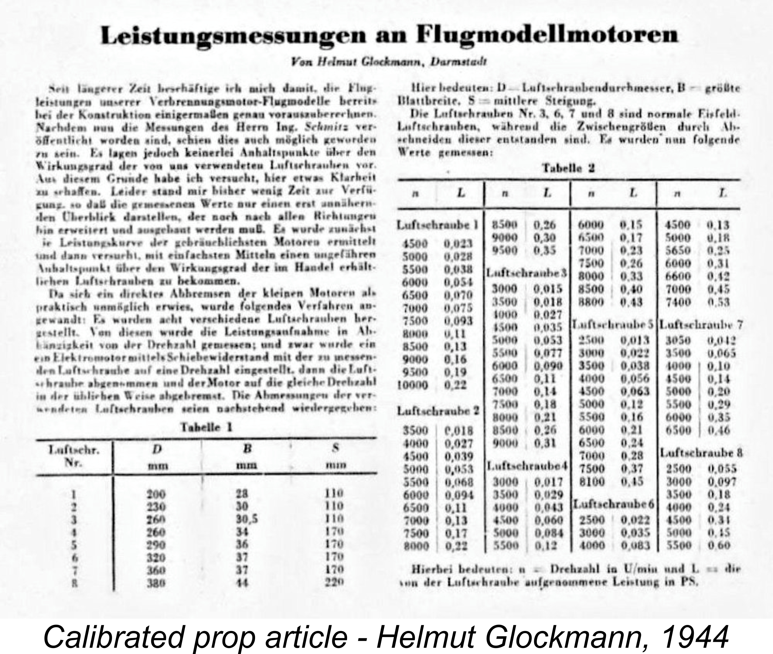 This concept was actually anticipated many years prior to its eventual adoption as a standard approach to the testing of model engines. My good mate Maris Dislers has reminded us of the often-overlooked fact that aeromodelling somehow managed to continue in Germany during WW2, to the extent that the German modelling magazine "Modellflug" continued in publication during those years (as did its British counterpart "Aeromodeller"). Issue no. 5/6 of Volume 9 of this publication (1944) included an article by Helmut Glockmann on the subject of model engine power output measurement using a standard set of calibrated airscrews.
 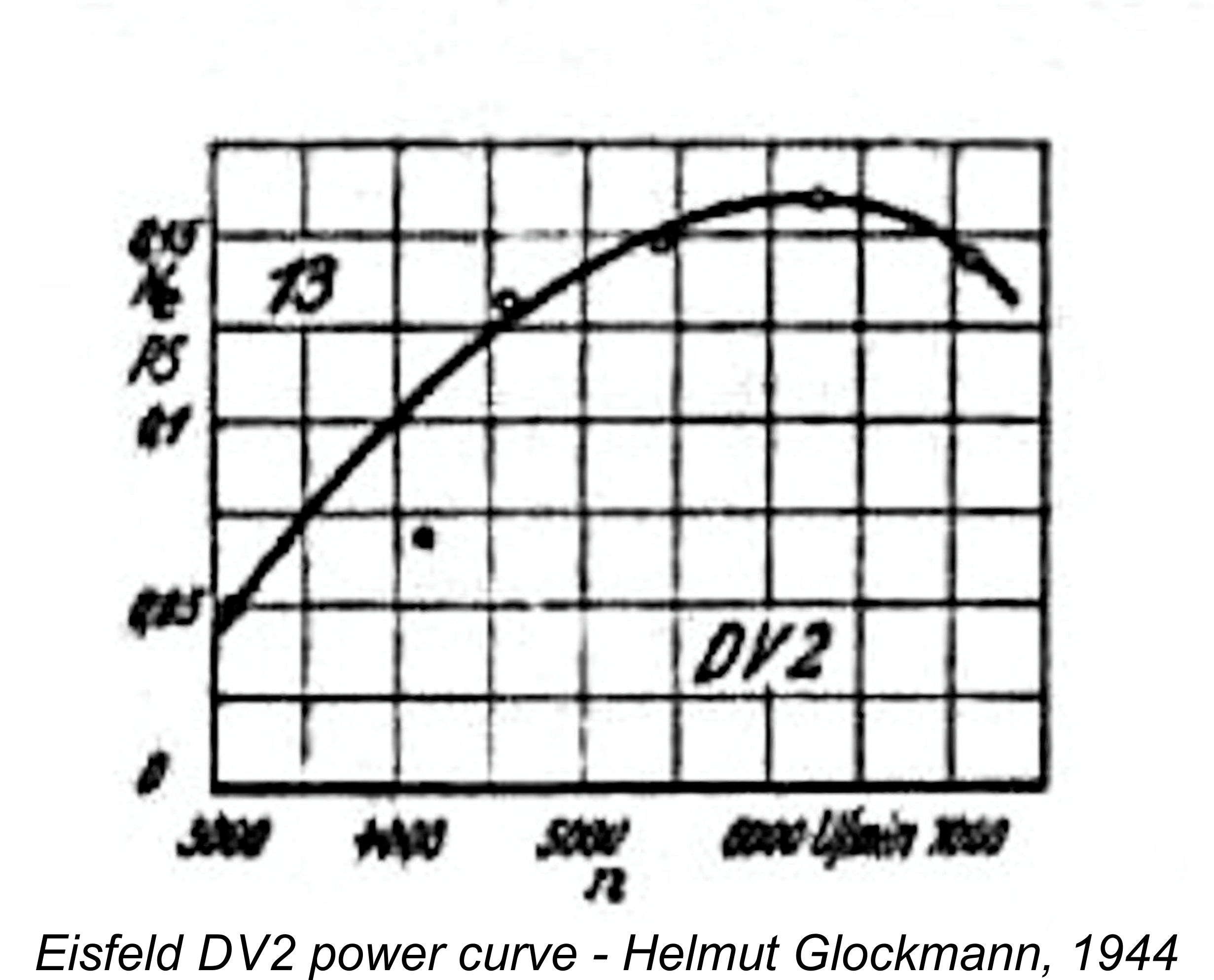 To illustrate the effectivenes of this method, Glockmann published power curves for several model engines which evidently remained available in Germany despite the intrusion of the war. He reported outputs of 0.16 BHP @ 6,200 rpm for the 2.5 cc (0.151 cuin.) Eisfeld DV2; 0.32 BHP @ 6,000 rpm for the 6 cc (0.366 cuin.) Eisfeld DV3; and 0.11 BHP @ 6,600 rpm for the Swiss Dyno of 2 cc (0.122 cuin.) displacement. These numbers generally appear to be quite credible.
 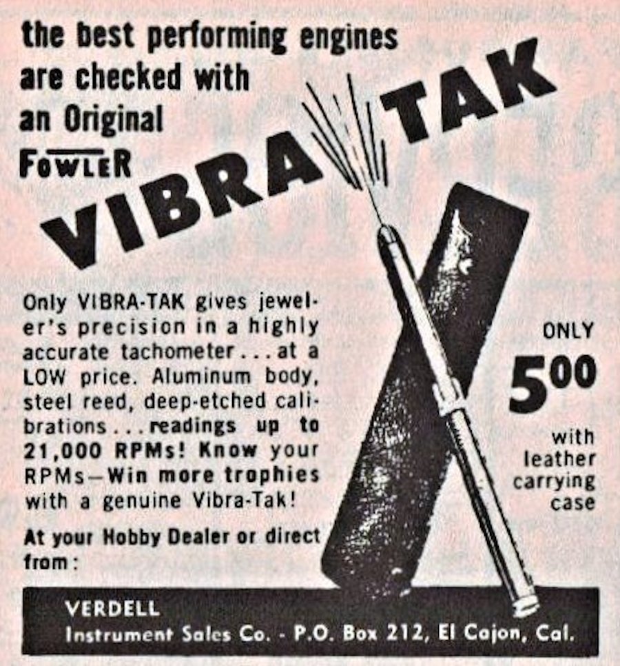 Moreover, during the pioneering era following the conclusion of WW2 there was no such thing as a standard range of airscrews for which dependable generic power curves could be developed. The method was of course perfectly practicable, but each individual tester would have had to create his own set of calibrated props.
 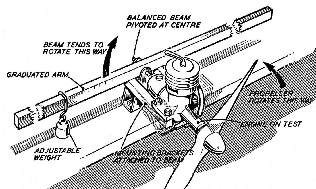 Now we don’t want the engine turning in response to this reactive torque – rather, we want the engine to remain in place while turning the airscrew! For this to happen, the mounting (or model) has to exert an equal and opposite reactive torque upon the engine to balance things out and maintain equilibrium between the engine and its mounting. Hence if we can measure the reactive torque that the mounting has to exert to keep the engine in position, we will have also measured the torque that the engine is applying to the airscrew. The direction of that measured torque is immaterial – it’s the actual figure that counts.
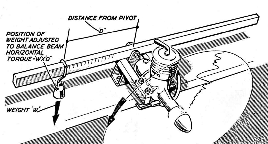 rearward extension of the engine’s central axis of rotation when in operation. An arm was fitted to this rig, and by hanging different weights from the arm (or moving the same weight to different positions on the arm) one could get a reading of the torque necessary to prevent the mounting from turning. This was theoretically equivalent to the torque being developed by the engine. Hopefully the attached figures taken from “Model Aero Engine Encyclopaedia” will make this clear.
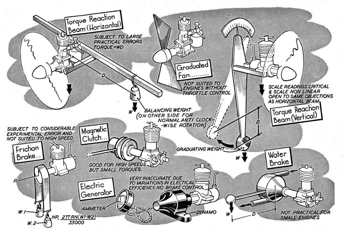 Heenan & Froude went through the various types of dynamometer then in current use, pointing out the advantages and disadvantages of each for the intended purpose. The attached figure from “Model Aero Engine Encyclopaedia” summarized the alternatives considered. The horizontal torque reaction beam was already familiar to “Aeromodeller” staff, as were its previously-discussed limitations. The vertical configuration of the same device (based upon the pendulum principle) had basically the same limitations to go along with a non-linear scale and extreme sensitivity to the smallest reading errors. The water brake approach was fine for full-sized engines but was not really considered a practical proposition for very small engines. Friction brakes were far too subject to errors and fluctuations, particularly at high speeds, due to temperature variations among other things. The dynamo method too was subject to major inconsistencies and errors due to changes in electrical efficiencies with temperature. Finally, the magnetic clutch system was only applicable for very small torque figures.
 As the rotor turns, the interaction of its induced magnetism combines with the magnetic field of the coil to cause the rotor to try to drag the coil around with it, exerting a torque equal to that being produced by the engine. The field coil is wrapped around a casing which is free to rotate around the axis of the system and would do so if it were not restrained by a balance arm and weight similar to that used in the old reaction cradle. The load, and hence the torque, can be adjusted on a continuous basis simply by varying the current passing through the coil, thus varying the strength of the applied magnetic field. Hopefully the attached figure extracted from “Model Aero Engine Encyclopaedia” will make this clear. In effect this is a very sophisticated variant of the magnetic clutch.
 The downsides are that the connection of a series of engines of widely differing sizes and outputs to the dynamometer is quite problematic in itself. Moreover, since there is no airscrew, some external means of engine cooling has to be arranged.
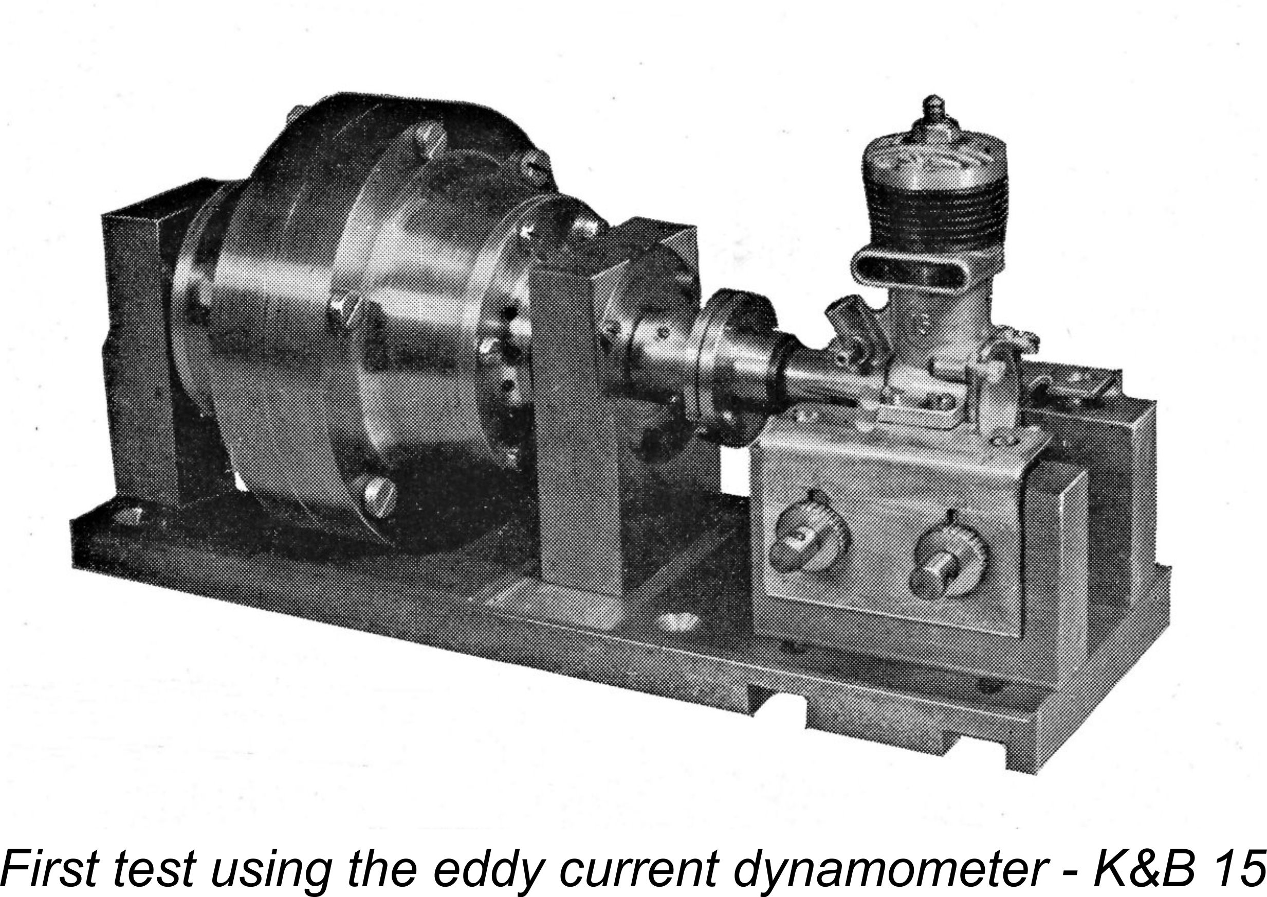 worked out. However, that was fine for “Aeromodeller” testing – what about the rest of us?? There was no way in which we were ever going to own our own dynamometers! Moreover, the practical hassles of using this equipment were simply unacceptable in a day-to-day modelling context.
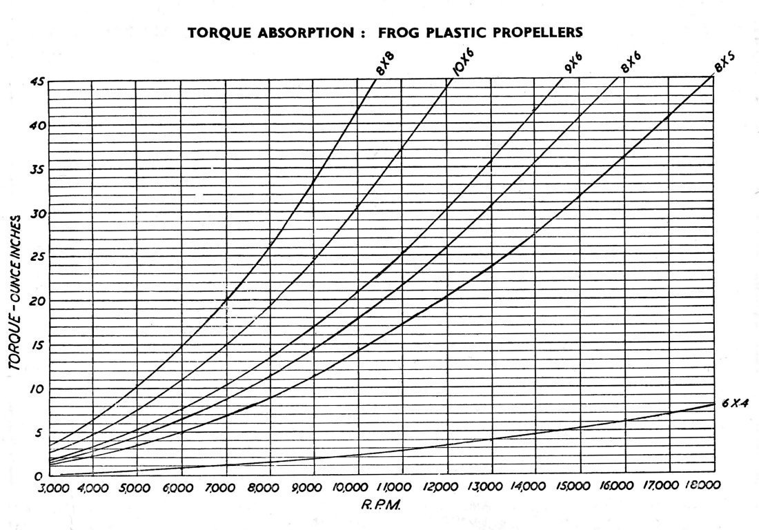 So there matters rested. Once some data was compiled from results obtained with the eddy current dynamometer, “Aeromodeller” did go so far as to publish torque absorption curves for certain ranges of commercial airscrews such as the FROG plastic series and the Stant range. However, they stressed that these curves could really only be considered as ball-park figures to assist modellers in selecting an appropriate airscrew for their engine. It was not until the advent of families of commercial airscrews which were produced to far higher standards of consistency that the possibility of using such airscrews to develop reasonably reliable power curves received renewed attention.
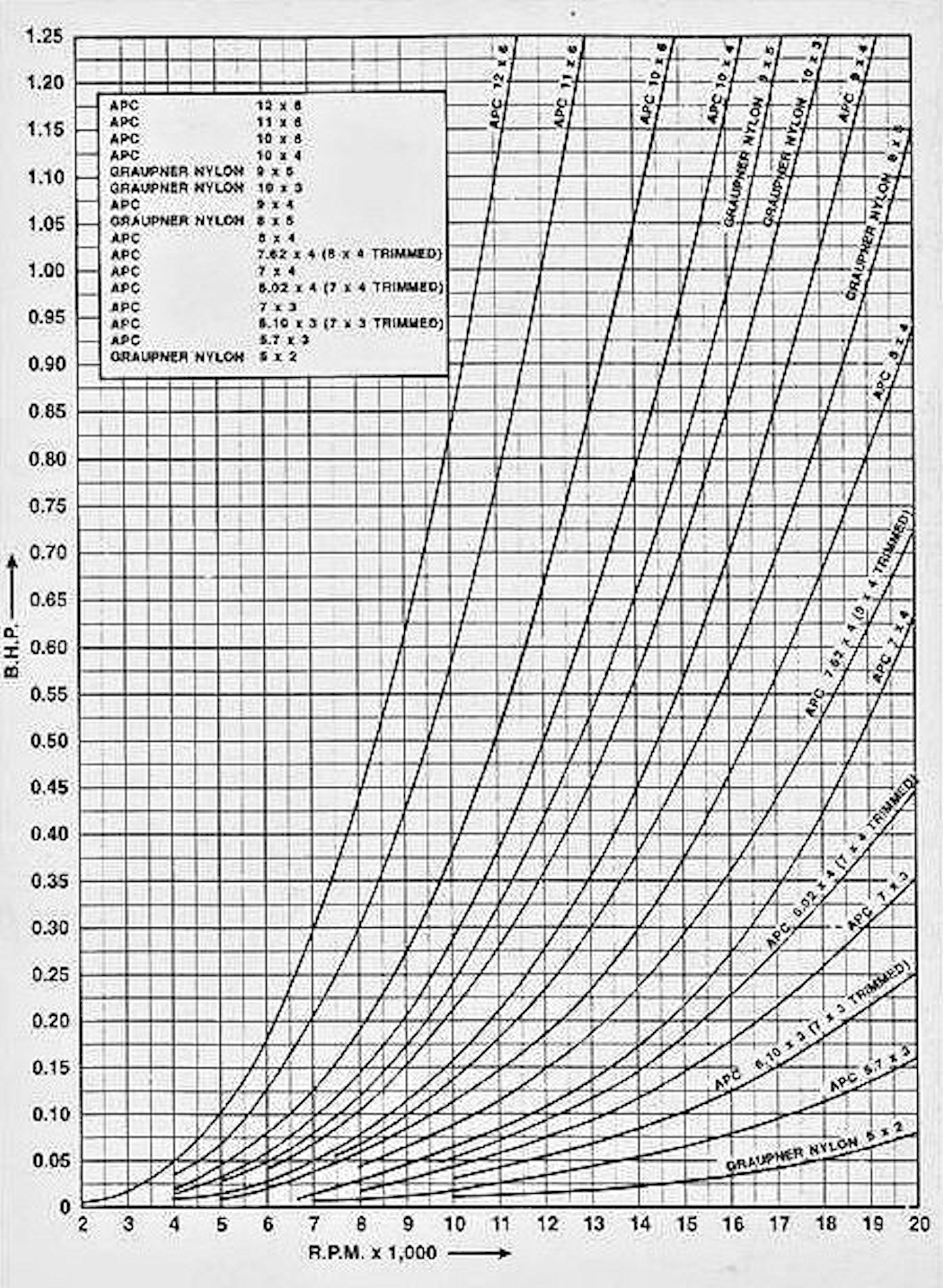 All well and good, but all of this was highly derivative, plus it took a very long time to get anywhere near right. Fortunately, the Editor of “Aeromodeller” magazine came to the rescue once again. Hearing from former David-Andersen distributor O. F. W. “Peter” Fisher that over in Norway Jan David-Andersen had designed and built a test rig to measure power absorption coefficients for different airscrews, the Editor contacted Jan to see if he could be persuaded to calibrate the set of test airscrews (APC and Graupner nylon) then being used by “Aeromodeller” engine tester Dick Roberts in the then-current series of model engine tests being published in the magazine. Jan was happy to oblige, the result being the set of curves which appear in the attached figure. My sincere thanks to my good mate David Owen for providing this table, which I did not have previously.
 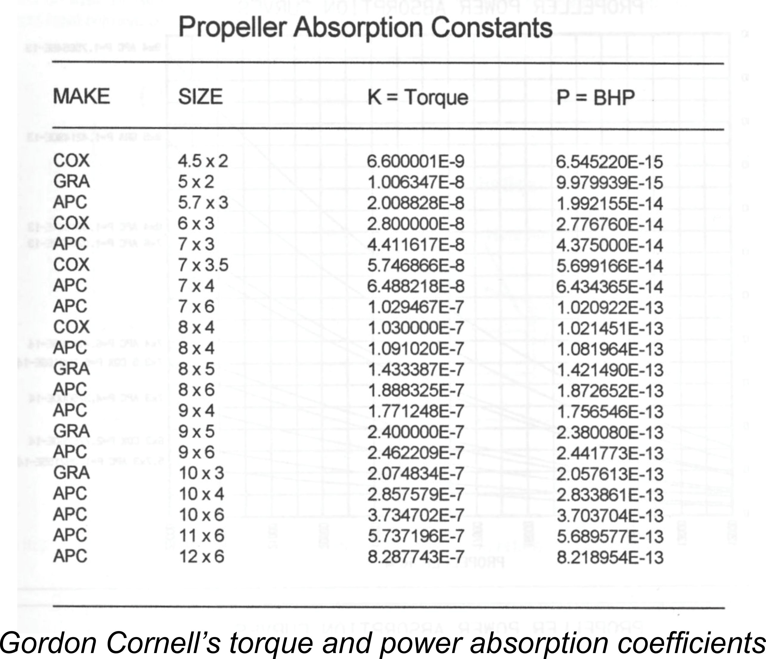 prop. Moreover, the accuracy to which you can establish and then measure the rpm for that prop will have a significant effect upon the accuracy of the derived power figure, since that figure varies with the cube of speed, as noted earlier.
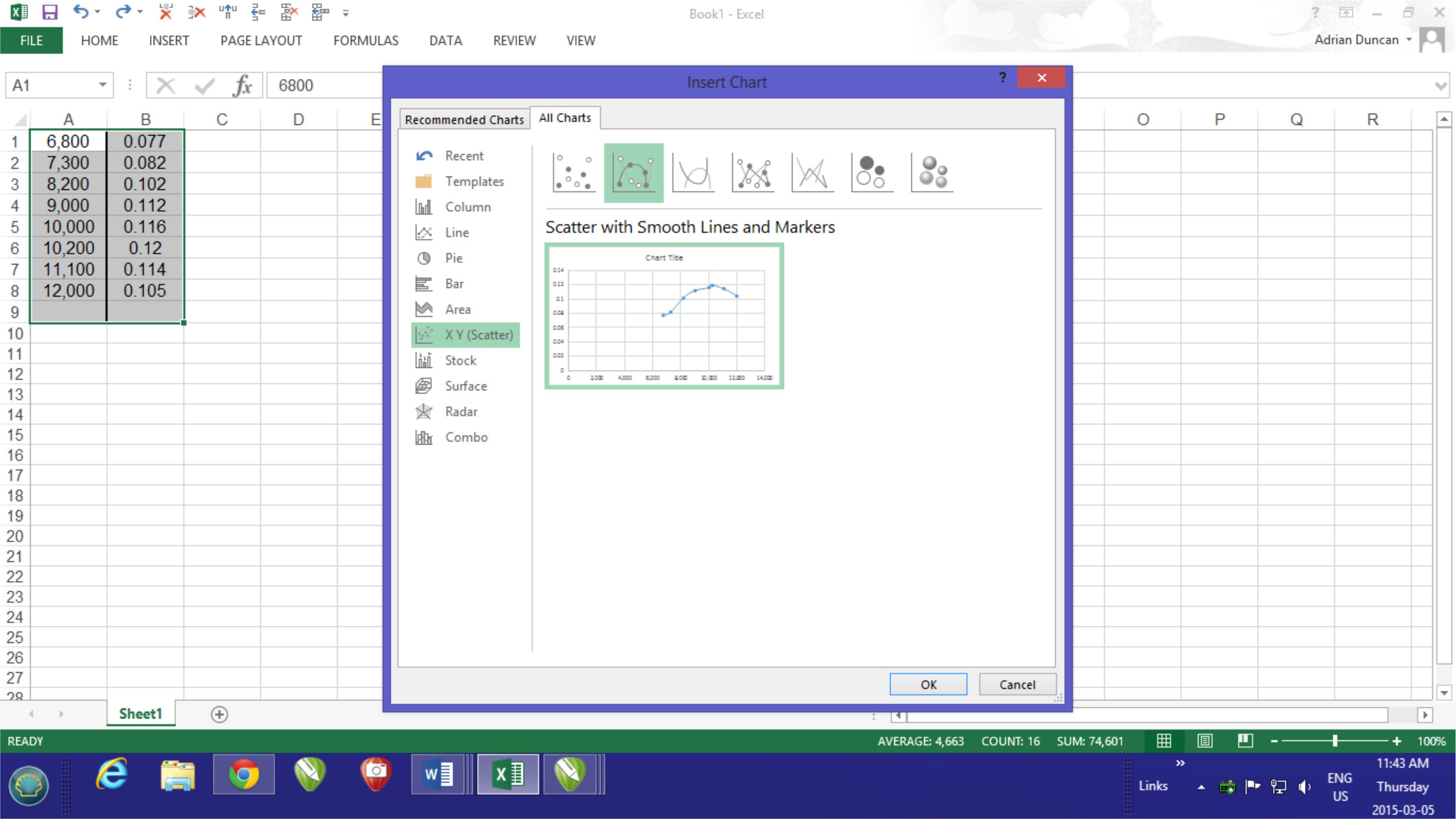 So how do you generate a power curve for your engine? Well, by far the easiest way is to paste the rpm data and calculated power figures into a bank Excel work-sheet. Highlight the two columns of figures and then click on "Insert" on the top tool-bar. This brings up another toolbar which includes a "Recommended Charts" option. Click on this, and a work-pane will appear which includes a rough chart showing your data in graphical form. You can improve the look of the graph by clicking "All Charts" at the top of the work-pane and then selecting "X Y Scatter" in the left-hand side menu and the "Smooth Line with Markers" option at the top. When the graph looks right, hit "OK" at the bottom right and there it is! You can format the axes and add a title at this stage. Then save the Excel doument, and you're done! A sample work-sheet of this kind is shown here.
 | |